Table of Contents
1. Introduction
Ever since I first started programming, I was always fascinated by noise functions. The idea that you can take a relatively simple algorithm and generate realistic-looking textures of clouds, fire, cloth, etc. is really cool.
However, as simple as the concept is, I still found myself struggling with putting it into code, until the idea one day clicked and I was able to finally implement it. To help others, who might wonder how this algorithm works, I'd like to share a small tutorial here how one might go about implementing a simple variant of Perlin noise in TypeScript.
One caveat of the code below is that it focuses more on readability, without paying much attention towards performance and optimization, and thus isn't exactly fast, despite the algorithm being Embarrasingly Parallel. For more serious implementations one should consider following the original algorithm's permutation lookup table-based approach, use WebGL with a fragment shader that can easily compute every point's noise value at the same time, or just use a better language than JS…
2. Basic outline
Given an arbitrarily sized rectangle, we need to do the following steps to fill it with noise:
- First we divide the rectangle into a grid of squares. The size of these squares is freely adjustable by us and it determines the general "roughness" of the result.
- For each of these grid points, we generate a so-called gradient vector. In the context of Perlin noise, these are little more than vectors whose magnitude is 1 and which point in random directions.
- Then, for every pixel inside the original rectangle, we gather the four closest grid-points and their accompanying gradients.
- We calculate the dot product of the vector formed by the pixel's coordinates and each of the gradients.
- To smush these values into one, we take a proportional part of both the upper and lower corners' values based on the X coordinate of our pixel and then calculate a final value from that based on the Y coordinate.
3. Implementation
3.1. Vector class
 1: class Vector {
 2:   x: number;
 3:   y: number;
 4:
 5:   constructor(x: number, y: number) {
 6:     this.x = x;
 7:     this.y = y;
 8:   }
 9:
10:   static random_gradient(): Vector {
11:     const angle = Math.random() * 2 * Math.PI;
12:     return new Vector(Math.cos(angle), Math.sin(angle));
13:   }
14:
15:   sub(other: Vector): Vector {
16:     return new Vector(this.x - other.x, this.y - other.y);
17:   }
18:
19:   add(other: Vector): Vector {
20:     return new Vector(this.x + other.x, this.y + other.y);
21:   }
22:
23:   dot_product(other: Vector): number {
24:     return this.x * other.x + this.y * other.y;
25:   }
26:
27:   toString(): string {
28:     return `(${this.x}, ${this.y})`;
29:   }
30: }
We begin by defining a very rudimentary Vector class. Usually we'd define more operations, like multiplication, length, etc., but for our purposes this suffices.1
You may wonder why we bother to define toString, when our end result will be graphical anyway. The reason is simple: We are going to associate data with our coordinates, using JavaScript's built-in Map. However, because these don't support indexing by objects, we need to first convert our Vector into a string, which does work as a key.2
3.2. Interpolation function
In our algorithm, every pixel's value comes from four different values, but the end result needs to be only a single value. Therefore we need a function that, when given two numbers, allows us to pick a third, that is a mix of a given percentage of one of our numbers and a complementary percentage of the other. For this we utilize Linear interpolation:
31: function lerp(percent: number, start: number, end: number): number {
32:   return start + percent * (end - start);
33: }
This function takes a [start, end] range and a percentage, and has the following properties:
lerp(0, start, end) = start + 0 * (end - start) = start,lerp(1, start, end) = start + 1 * (end - start) = start + end - start = end,- Otherwise,
lerp(x, start, end) = ((1 - x) * start) + (x * end).
Example: Let's say our inputs are 0.25, 1, and 5. We add to 1 a fourth of the difference between 5 and 1, thus get 1 + 0.25 * (5 - 1) = 1 + 0.25 * 4 = 1 + 1 = 2. If we were to pick 0.5 as our percent instead, our result would be 3 which is the exact middle between 1 and 5.
This already works, but it's less than ideal because the edges of the interpolation function are very sharp leading to very obvious artifacts on the edges of grid cells:
Figure 1: Noise full of visual artifacts.
It's easy to see why this happens if we take a look at how interpolating between some random values looks like:
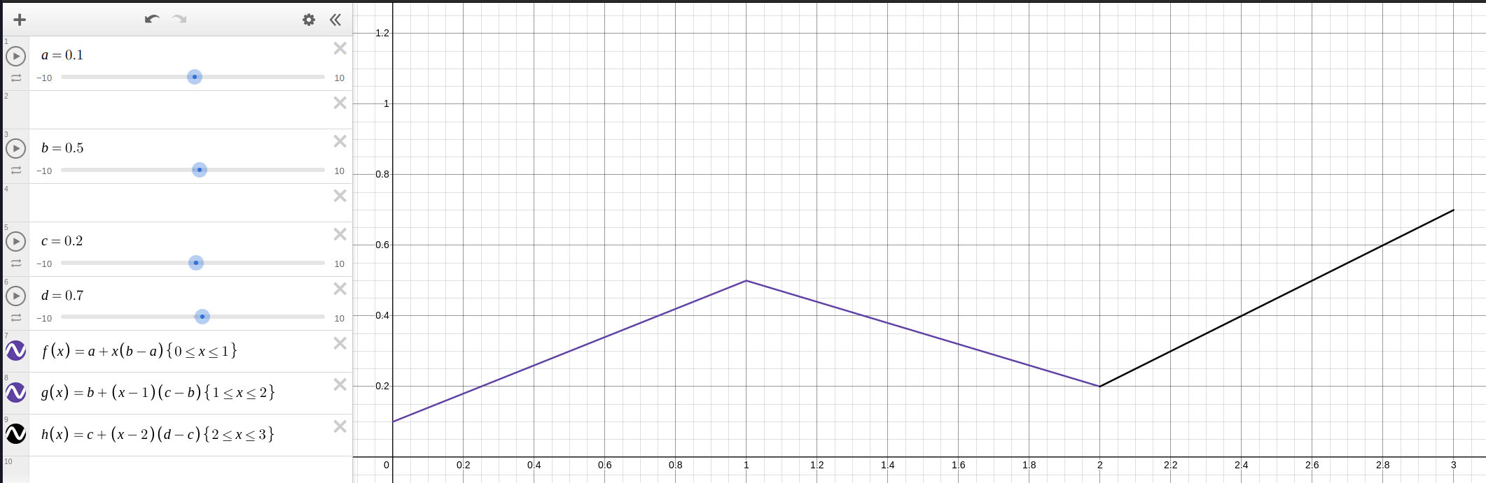
Figure 2: Sharp peaks and valleys that show up as visible lines in our noise.
Thankfully fixing this is fairly simple. If the issue is that the endpoints' connections are too sharp, we simply have to smoothen them out. Enter the "Smoothstep" function:
34: function smoothstep(x: number): number {
35:   return 6*x**5 - 15*x**4 + 10*x**3;
36: }
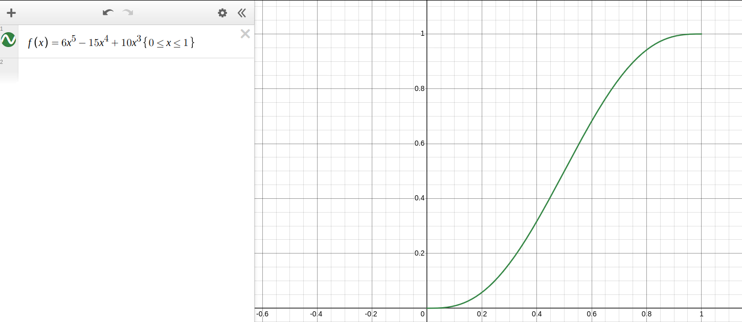
Figure 3: The Smoothstep function visualized in the range [0, 1].
Given a number between [0, 1], this function returns another value between [0, 1], but "smoothened out". To provide a better visual explanation of what this means, let's see the previous interpolation, after we ran our percentages through Smoothstep:
37: function interpolate(percent: number, start: number, end: number): number {
38:   const smooth_percent = smoothstep(percent);
39:   return lerp(smooth_percent, start, end);
40: }
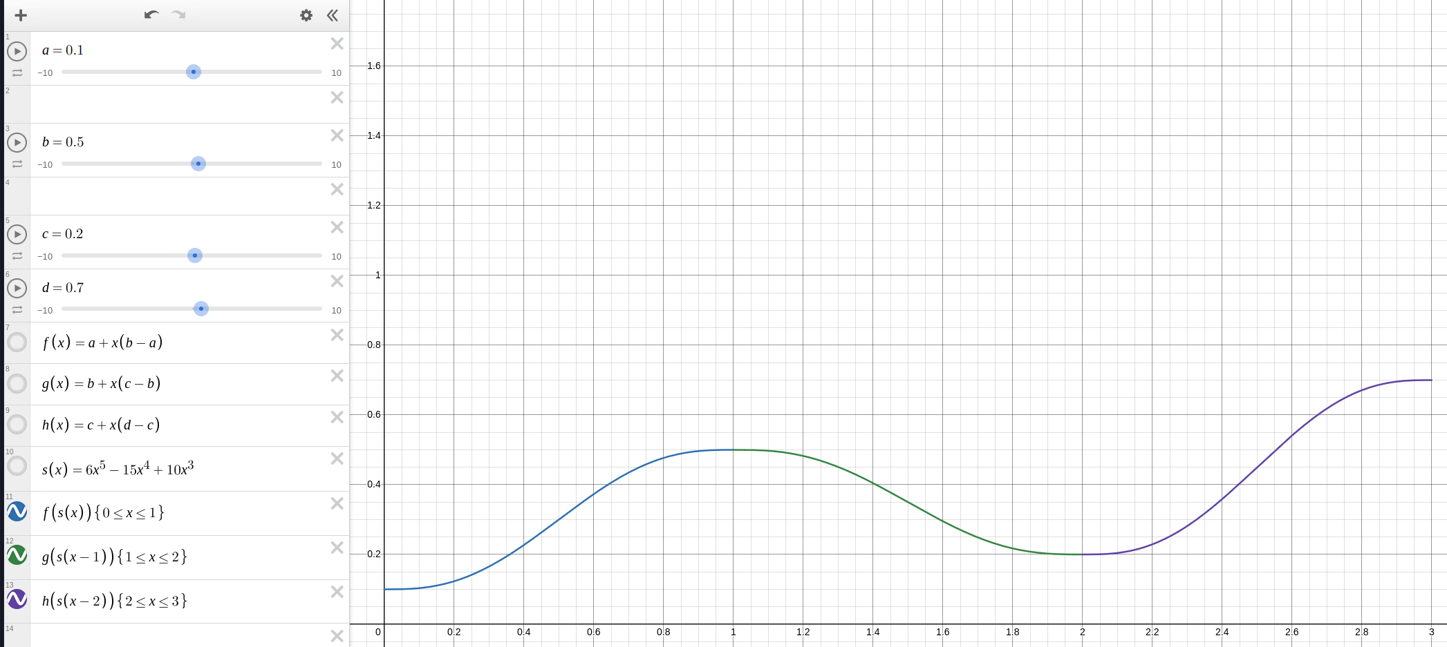
Figure 4: The peaks and valleys are gone.
As you can see, the end result looks a lot more "natural" as one curve flows nicely into the next, without any obvious edges.
3.3. Noise function
With all the groundwork finally done, we reach the main algorithm. Let's take it in parts:
41: const gradients = new Map<string, Vector>();
42:
43: function get_gradient(vec: Vector): Vector {
44:   const key = vec.toString();
45:   let gradient: Vector | undefined = gradients.get(key);
46:
47:   if (!gradient) {
48:     gradient = Vector.random_gradient();
49:     gradients.set(key, gradient);
50:   }
51:
52:   return gradient
53: }
First we initialize a Map to hold our calculated gradients. This both serves as an optimization (we only need to calculate a gradient for every grid cell corner once) and also ensures that every corner always gets the same gradient (our random_gradient function has no knowledge about the outside state of our function, so it'll happily generate as many random vectors as we ask for).3
55: const offset_vectors: Vector[] = [
56:     new Vector(0, 0),
57:     new Vector(1, 0),
58:     new Vector(0, 1),
59:     new Vector(1, 1),
60: ];
We then create four offset vectors, which will help us address the grid cell's corners.
62: function noise(x: number, y: number): number {
63:   const coordinate_vector = new Vector(x, y);
64:   const floored_vector = new Vector(Math.floor(x), Math.floor(y));
65:   const fraction_vector = coordinate_vector.sub(floored_vector);
Our function takes in an X,Y pair representing the coordinates of a pixel. This pair is turned into three separate vectors:
- one for the raw coordinates (
coordinate_vector), - one for the grid cell (
floored_vector), - and finally the relative position of the coordinates inside the grid cell (
fraction_vector),
66:   // top left, top right, bottom left, bottom right
67:   const [tl, tr, bl, br] = offset_vectors.map((offset_vector) => {
68:     const corner_vector = floored_vector.add(offset_vector);
69:     const gradient = get_gradient(corner_vector);
70:
71:     return coordinate_vector.sub(corner_vector).dot_product(gradient);
72:   });
Next we calculate the dot products between the vector of our pixel's coordinates and each corner's gradient. get_gradient ensures we always get the same gradient for a given corner.
73:   const upper_interpolation = interpolate(fraction_vector.x, tl, tr);
74:   const lower_interpolation = interpolate(fraction_vector.x, bl, br);
75:
76:   const noise_value = interpolate(
77:     fraction_vector.y,
78:     upper_interpolation,
79:     lower_interpolation,
80:   );
81:
82:   return noise_value;
83: }
84:
Finally we do a 2D interpolation using the function we defined earlier. We first interpolate between the ranges of [top left, top right] and [bottom left, bottom right] using the pixel coordinate's relative X position, and then, with one final interpolation using the coordinate's relative Y position, we get our noise value.
3.4. Main loop
 85: function generate_noise(
 86:   width: number,
 87:   height: number,
 88:   resolution: number
 89: ): Float32Array {
 90:   gradients.clear();
 91:
 92:   const values = new Float32Array(width * height);
 93:
 94:   for (let y = 0; y < height; y++) {
 95:     for (let x = 0; x < width; x++) {
 96:       const x_percent = x / width;
 97:       const y_percent = y / height;
 98:
 99:       const value = noise(
100:         x_percent * resolution,
101:         y_percent * resolution,
102:       );
103:
104:       // Map [-1, 1] => [0, 1]
105:       values[y * width + x] = (value + 1) / 2;
106:     }
107:   }
108:
109:   return values;
110: }
First we clear the gradients map, as we don't want any previous data to interfere in case this isn't the first time we run the function.
Then we iterate through every pixel in our rectangle and calculate its coordinates, mapping [0, width] and [0, height] to [0, 1]. We also take a parameter called resolution, this determines how "zoomed in" our noise looks like:
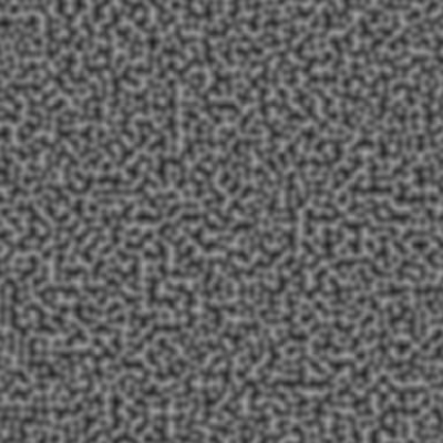
Figure 5: Noise with high resolution value.

Figure 6: Noise with low resolution value.
Finally, our noise function returns values in the range of [-1, 1], but we need [0, 1], so we add one to our result, mapping it to [0, 2] and then divide it by 2, thus end up with [0, 1].
111: document.getElementById("button").addEventListener("click", () => {
112:   const canvas = document.getElementById("canvas") as HTMLCanvasElement;
113:   const ctx = canvas.getContext("2d");
114:
115:   const maxFactor = Number(
116:     (document.getElementById("factor") as HTMLInputElement).value
117:   );
118:
119:   const baseFrequency = Number(
120:     (document.getElementById("frequency") as HTMLInputElement).value
121:   );
122:
123:   const width = canvas.width;
124:   const height = canvas.height;
125:   const imageData = ctx.getImageData(0, 0, width, height);
126:
127:   imageData.data.fill(0);
128:
129:   for (let factor = 0; factor <= maxFactor; factor++) {
130:     const values = generate_noise(width, height, baseFrequency * (2 ** factor));
131:
132:     for (let y = 0; y < height; y++) {
133:       for (let x = 0; x < width; x++) {
134:         const idx = y * width + x;
135:         const value = values[idx];
136:         const color = Math.floor(Math.max(0, value) * 255 / (2 ** (factor + 1)));
137:
138:         imageData.data[idx * 4 + 0] += color / 1.5;
139:         imageData.data[idx * 4 + 1] += color / 1.3;
140:         imageData.data[idx * 4 + 2] += color;
141:         imageData.data[idx * 4 + 3] = 255;
142:       }
143:     }
144:   }
145:
146:   ctx.putImageData(imageData, 0, 0)
147: });
Since I don't want to cause lag immediately on page load, I bound the noise generation to a button that you can find below. We request the underlying image data from our canvas element and zero it out. This is done as a precaution in case the user presses the button multiple times. Without this reset, the += operations below would quickly oversaturate our output image.
For this demo, I added two user-controlled variables, these being factor, which determines how many layers of noise we generate and baseFrequency, which determines the initial resolution (i.e. roughness) of the noise. For some examples, try a factor of 8 and frequency of 1 for a gentle fog and 4 and 16 for a fuzzy carpet.
We generate a noise array with the given iteration's frequency and fill in the current pixel based on the value of the noise. I skewed the numbers a little to get a pleasant blue color, without any modification, we'd be left with a grayscale image.
Thank you for reading this post and I hope you may have learned something fun! If you'd like to read the code as a whole, you can access it here.
Footnotes:
In fact, we could easily get away without a class and just use inlined operations with either {x: number, y: number} objects or [x, y] arrays, but I believe the class-based version provides most pedagogical clarity, so that's the one I went with.
Technically the Map really doesn't care what we pass in as key. But since all keys are coerced into primitives, all of our Vector-s would be turned into strings in the form of the dreaded "[object Object]" and lose their identity, which would pretty much defeat the point of a hash-map. To avoid this, we override toString and instead return a sensible and, more importantly, unique string representation, that our map can take with no issue.
Those who are already familiar with the algorithm (or just read its Wikipedia page before continuing this article) might have realized that this is a vastly different way of generating gradients compared to the original version.
In the original we only have a handful (8 or 16) pre-generated gradient vectors and we pick one of them based on a somewhat involved process of hashing the current coordinate and then chopping off the lower 4 bits of the resulting number. While this most likely results in faster code, I find that it somewhat obscures of what we're really doing.